Process Amplicon Sequencing Data

Login to NASA EDGE

1. Navigate to the NASA EDGE platform by going to https://nasa-dev.edgebioinformatics.org/

2. Follow steps 2 - 5 of the Setup a NASA EDGE Account instructions to login to the NASA EDGE platform.

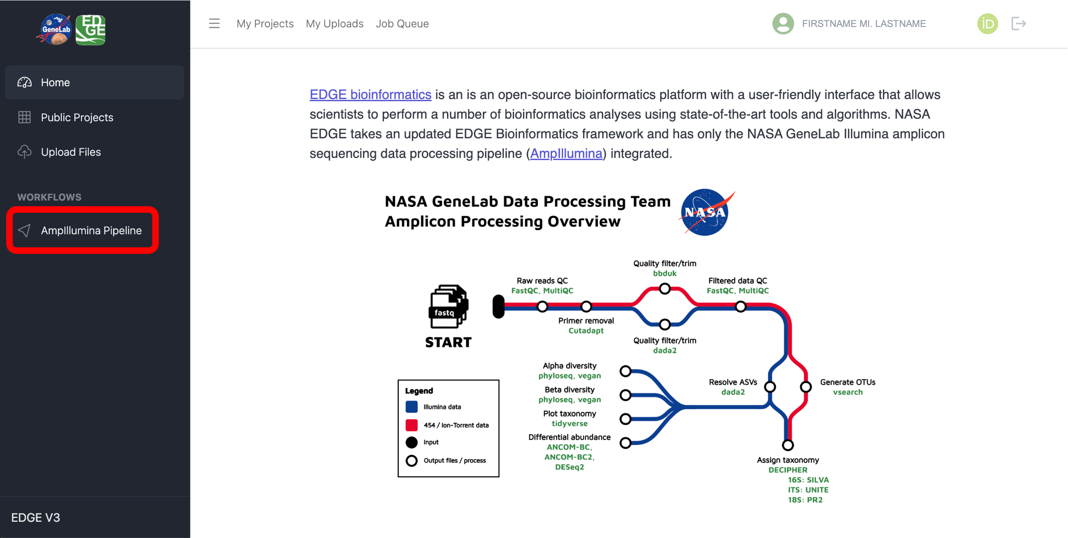
3. Once logged into the NASA EDGE platform, click on “AmpIllumina Pipeline” under “WORKFLOWS” in the side bar menu as shown below:

4. To process an amplicon sequencing dataset hosted on the NASA Open Science Data Repository (OSDR), follow the Process an OSD dataset instructions below.

5. To process a non-OSD dataset, such as your own data or a dataset shared on the NASA EDGE platform, follow the Process a non-OSD dataset instructions below.

Process an OSD dataset

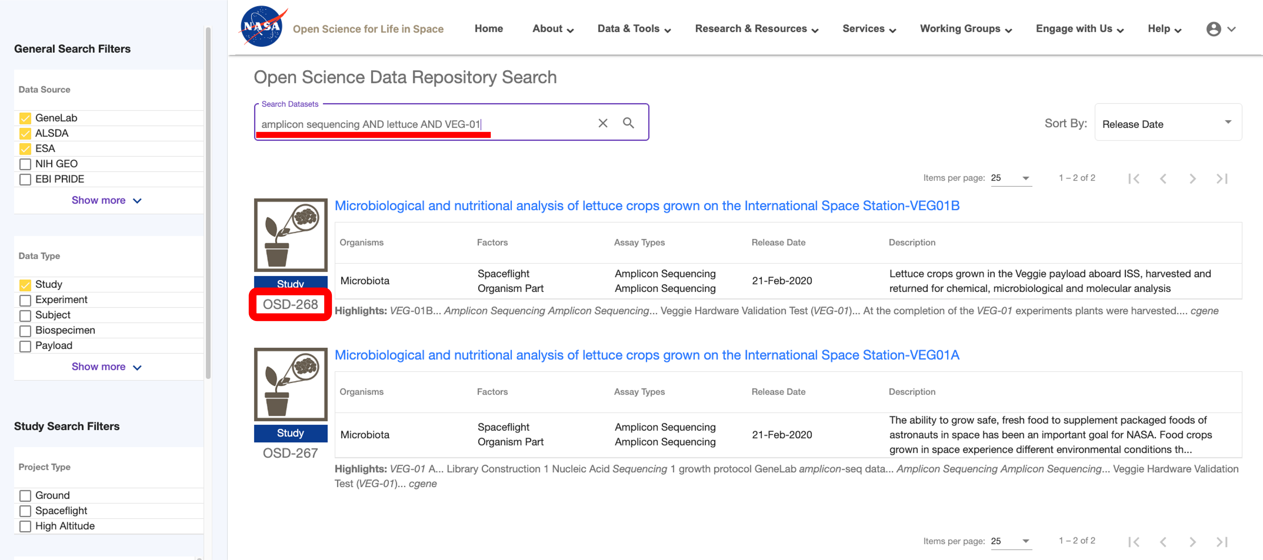
1. To process a dataset hosted on OSDR, navigate to the OSDR repository and search for the amplicon sequencing dataset you want to process using the free text search bar at the top of the page. Note the OSD number of the dataset you want to process as shown below:

   Note: If you are unfamiliar with OSDR, visit the OSDR Tutorials page to learn how to Access Data in the Open Science Data Repository and how to Navigate an OSDR Study Page.

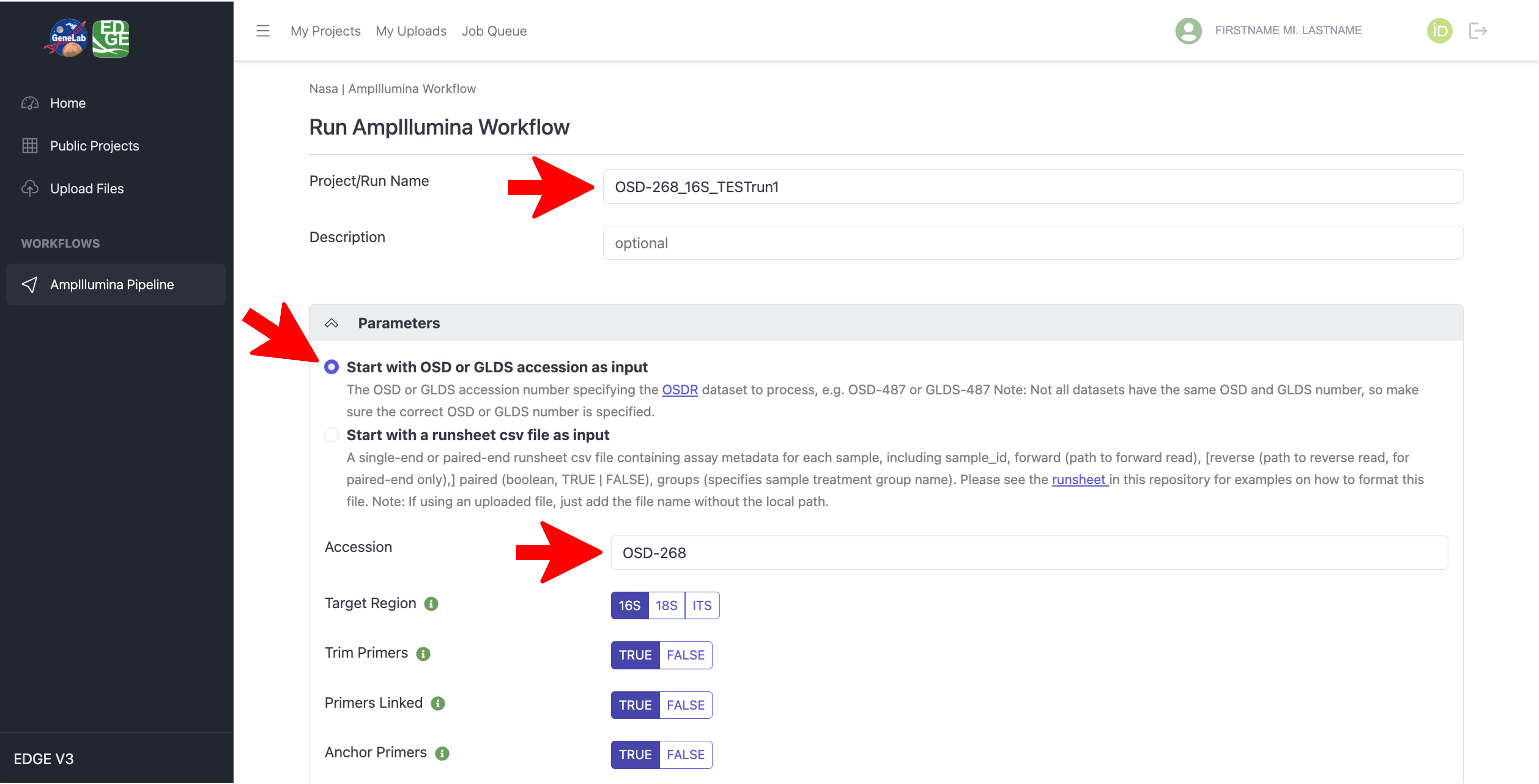
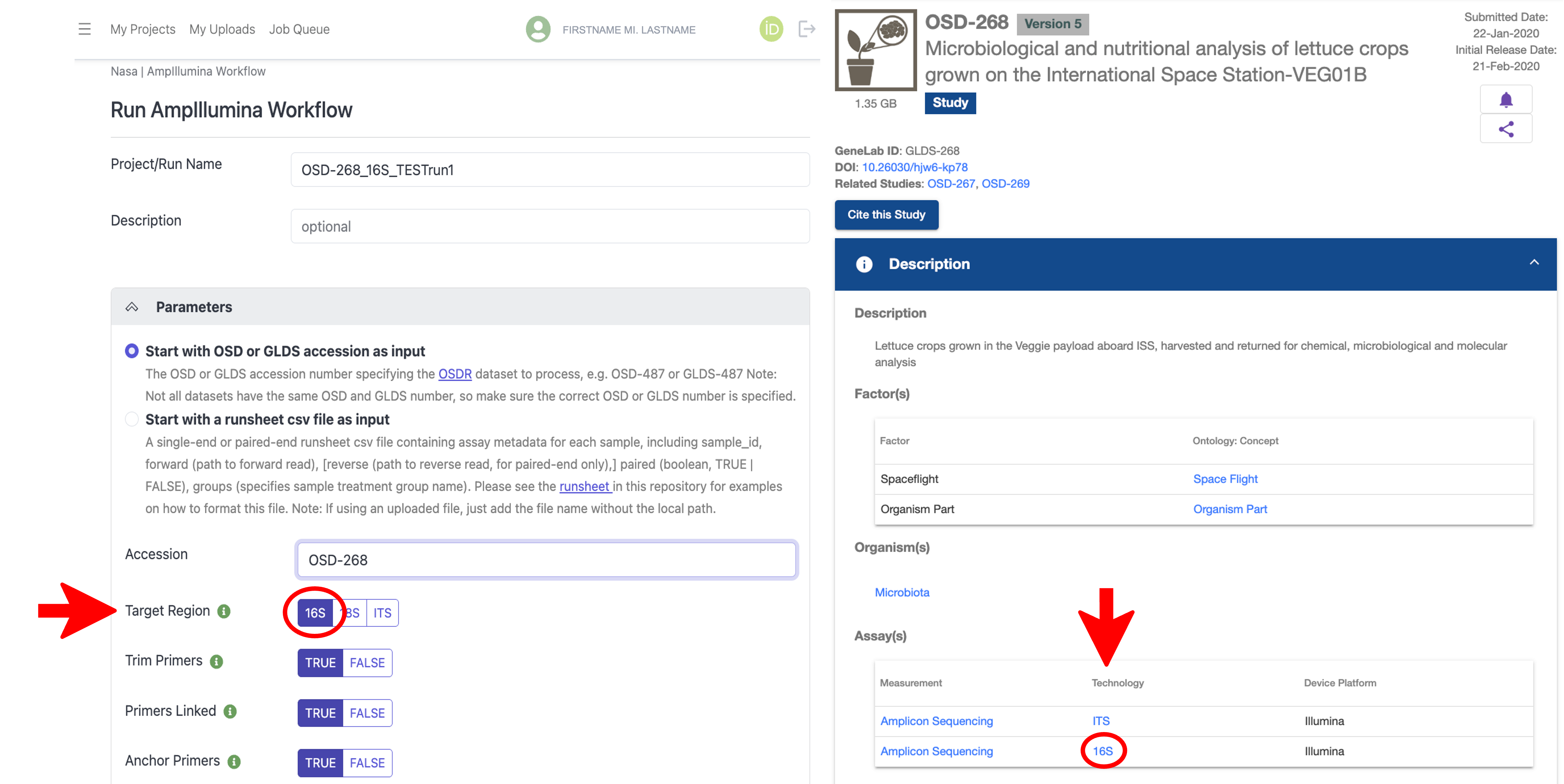
2. With the AmpIllumina Workflow selected in the NASA EDGE platform, type in a Project/Run Name for your project (required) and an optional Description, then under the “Parameters” section, select “Start with OSD or GLDS accession as input”, and in the Accession text box, type in the OSD number you want to process as shown below:

3. Under the “Parameters” section, select the amplicon Target Region used for processing, which can be found on the OSD study page under Assay(s) -> Technology for the select dataset as shown below:

   Note that some amplicon sequencing datasets on OSDR contain multiple sets of sequencing data, each with a different amplicon target region used, so be sure to select the target region you want to process on the NASA EDGE platform.

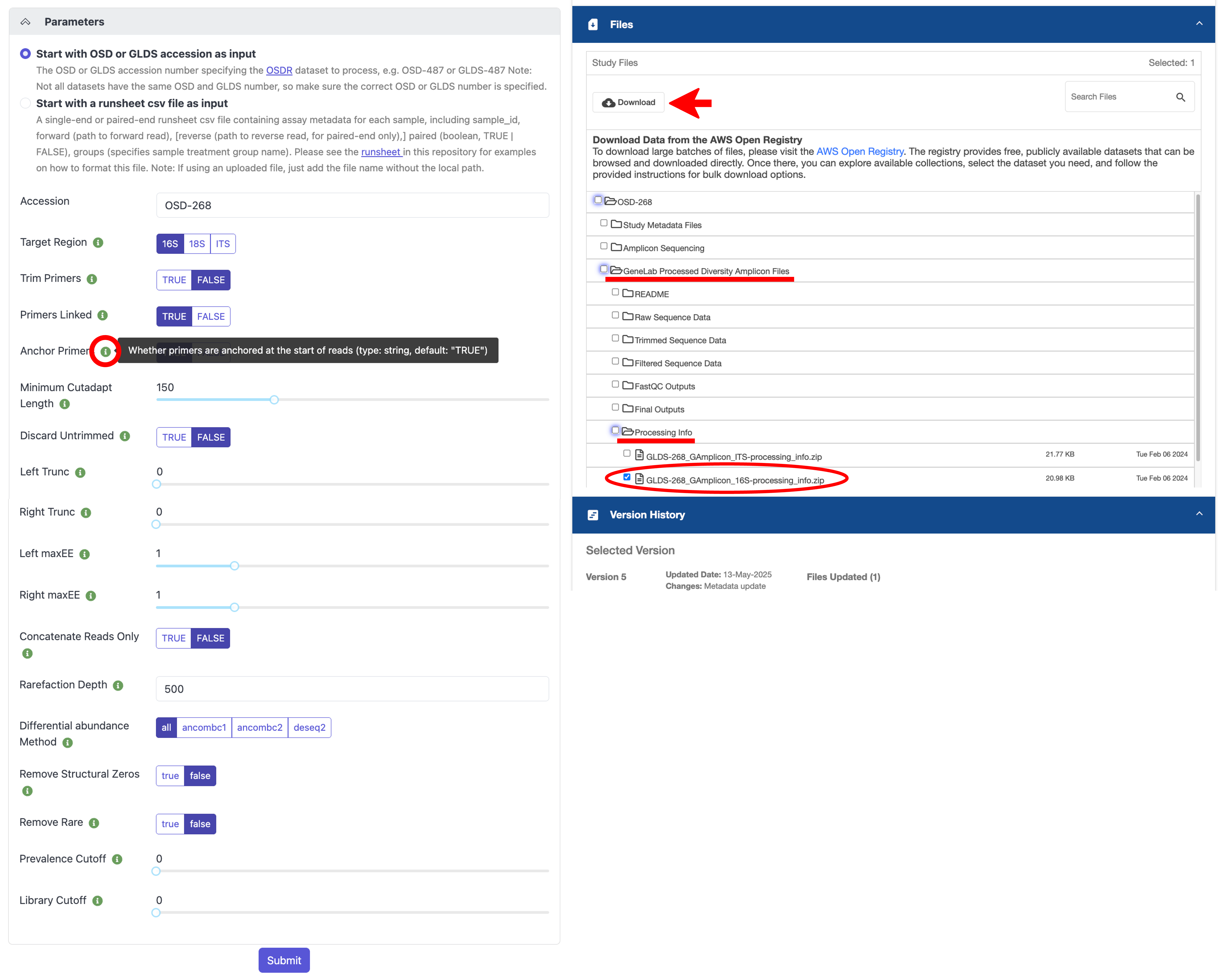
4. All other parameters are set to default values but can be modified. If you are unsure what a specific parameter does, hover over the green “i” icon next to the parameter name for more information, as shown below. If you want to re-process an OSD dataset using the exact parameters that were used to generate the GeneLab processed data on the OSDR repository, the parameter values used can be found in the processing info directory on the OSD study page, which can be downloaded under Files -> GeneLab Processed Diversity Amplicon Files -> Processing Info -> *processing_info.zip, as shown below.

   Note that the parameters values in the example below were set to match what was used to generate the processed data for this dataset in the OSDR repository.

5. When you are satisfied with your parameter selection, click the “Submit” button at the bottom to submit your job to the processing queue.

6. To check the status of your submitted job, following the instructions in the Track, Share, and Modify Projects tutorial.

7. Once your job is complete, you can view and download all output files and visualizations by following the instructions in the View and download output files section below.

Process a non-OSD dataset

1. To process a dataset that is not hosted on OSDR, such as your own amplicon sequencing data, you’ll first need to create a runsheet csv file that contains the metadata required for processing amplicon sequence datasets through the GeneLab amplicon Illumina sequencing data processing pipeline (AmpIllumina), as specified here.

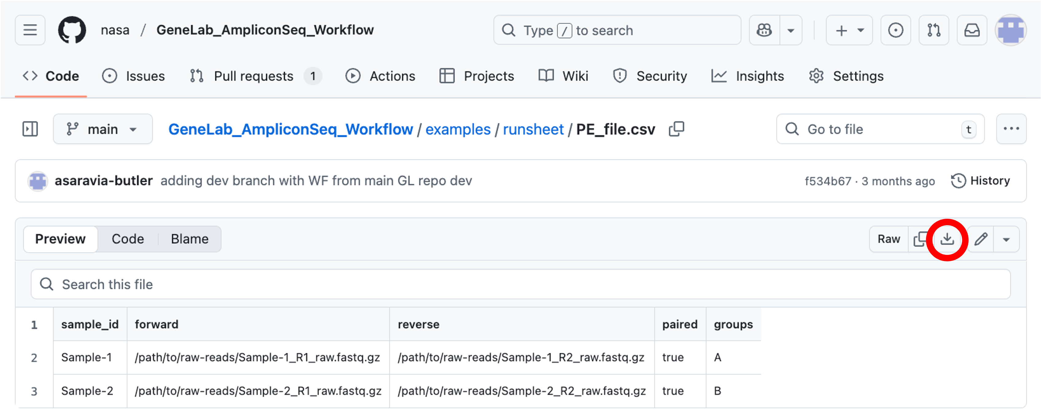
2. To ensure the runsheet format is correct, it is recommended to download the example runsheet PE_file.csv file for paired-end data or the SE_file.csv file for single-end data from GitHub by clicking on the download link as shown below:

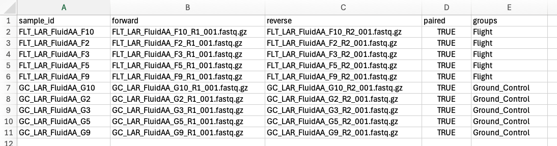
3. Open the example runsheet on your local computer and fill in the metadata columns with your sample info. A description of what should be included in each column can be found on GitHub here. An example of a completed runsheet csv file for a paired-end dataset is shown below:

   Note: The “forward” and “reverse” (PE data only) columns should only include the forward and reverse fastq file names, respectively, for each respective sample. Make sure the sample, file, and group names do not contain any spaces or weird characters.

4. Save your completed runsheet as a csv file.

5. Upload your runsheet csv file and your forward and reverse (for PE datasets only) fastq files to the NASA EDGE platform by following the “Upload data” instructions in the Setup a NASA EDGE Account guide.

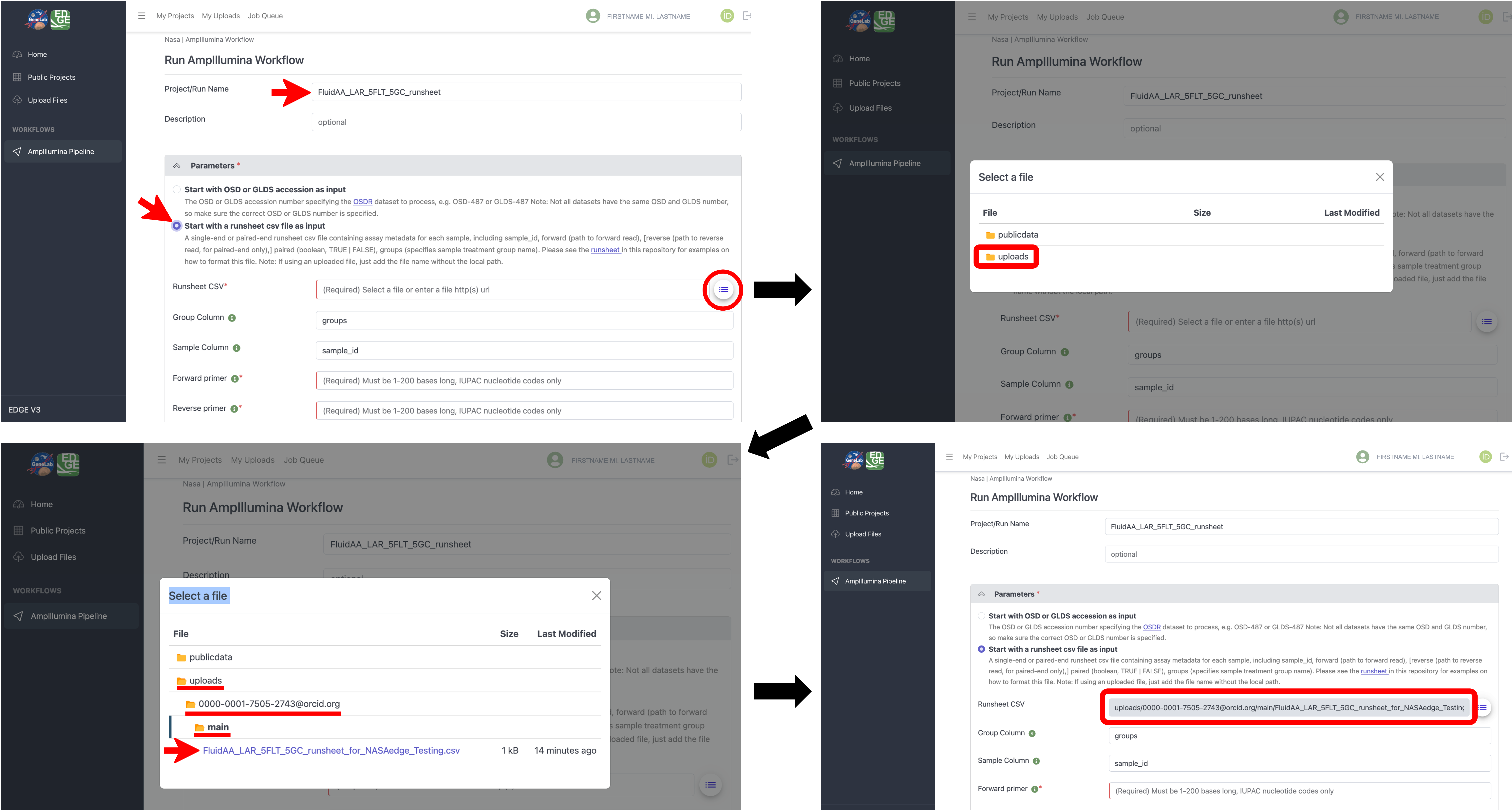
6. Once your runsheet and fastq files are successfully uploaded, navigate to the AmpIllumina workflow on the NASA EDGE platform and type in a Project/Run Name for your project (required) and an optional Description, then under the “Parameters” section, select “Start with a runsheet csv file as input”, and for the “Runsheet CSV” parameter, click on the drop-down icon to open the “Select a file” window as shown below. In the “Select a file” pop-up windown, you can select the “publicdata” folder to access publicly available datasets or you can navigate to your uploaded files by selecting the “uploads” folder -> your orcid folder -> then the “main” folder. Once in the main folder you will see all CSV files that you have uploaded to the platform. Select the runsheet csv file you uploaded in step 5. You will then see the selected runsheet populate the “Runsheet CSV” parameter of the workflow as shown below.

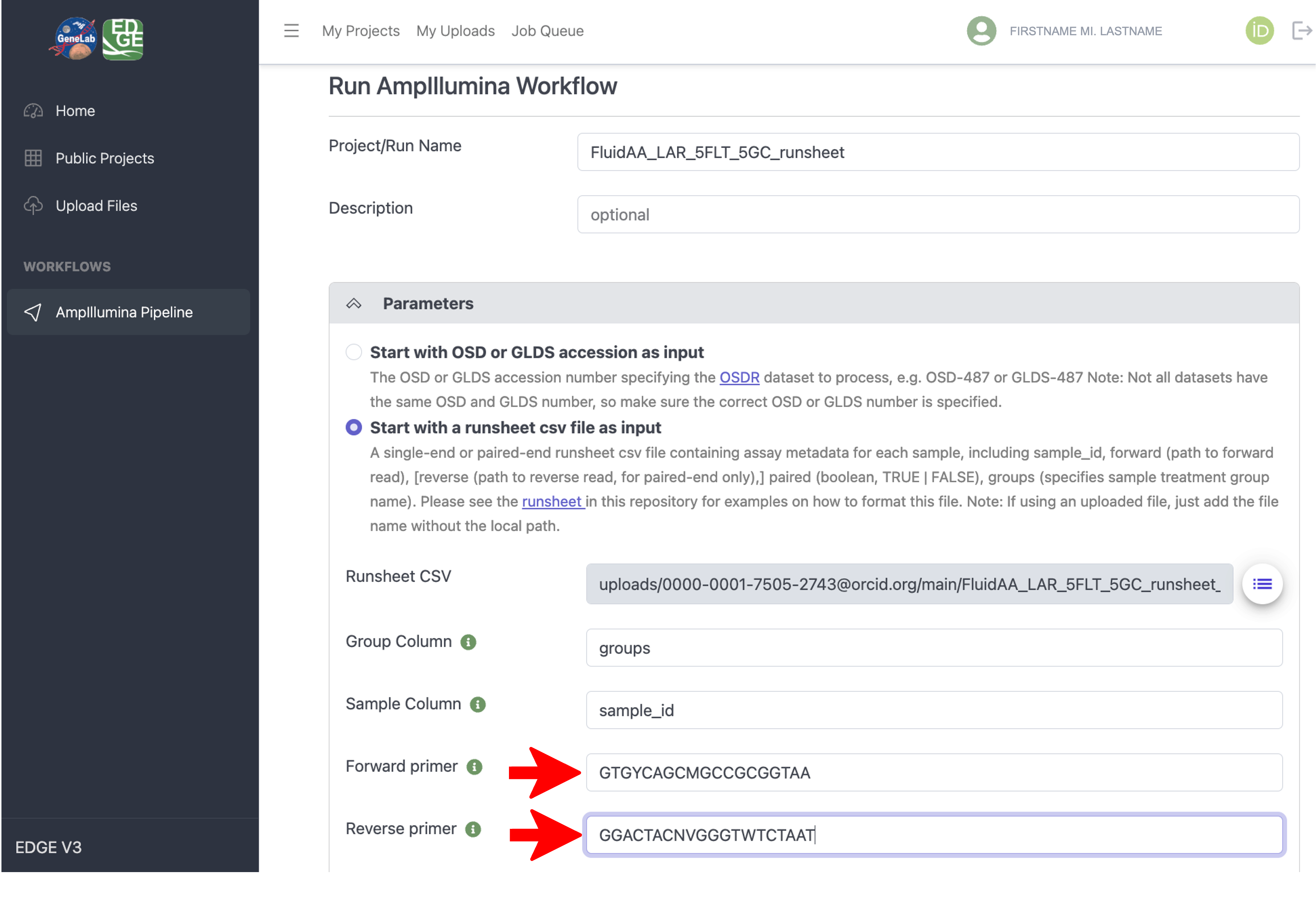
7. Next, input the forward and reverse primer sequences used to amplify the amplicon that was sequenced in your dataset, as shown in the example below.

   Note that the “Group Column” and “Sample Column” parameters will only need to be modified if you did not use the example runsheet csv file specified in steps 1 - 3 above.

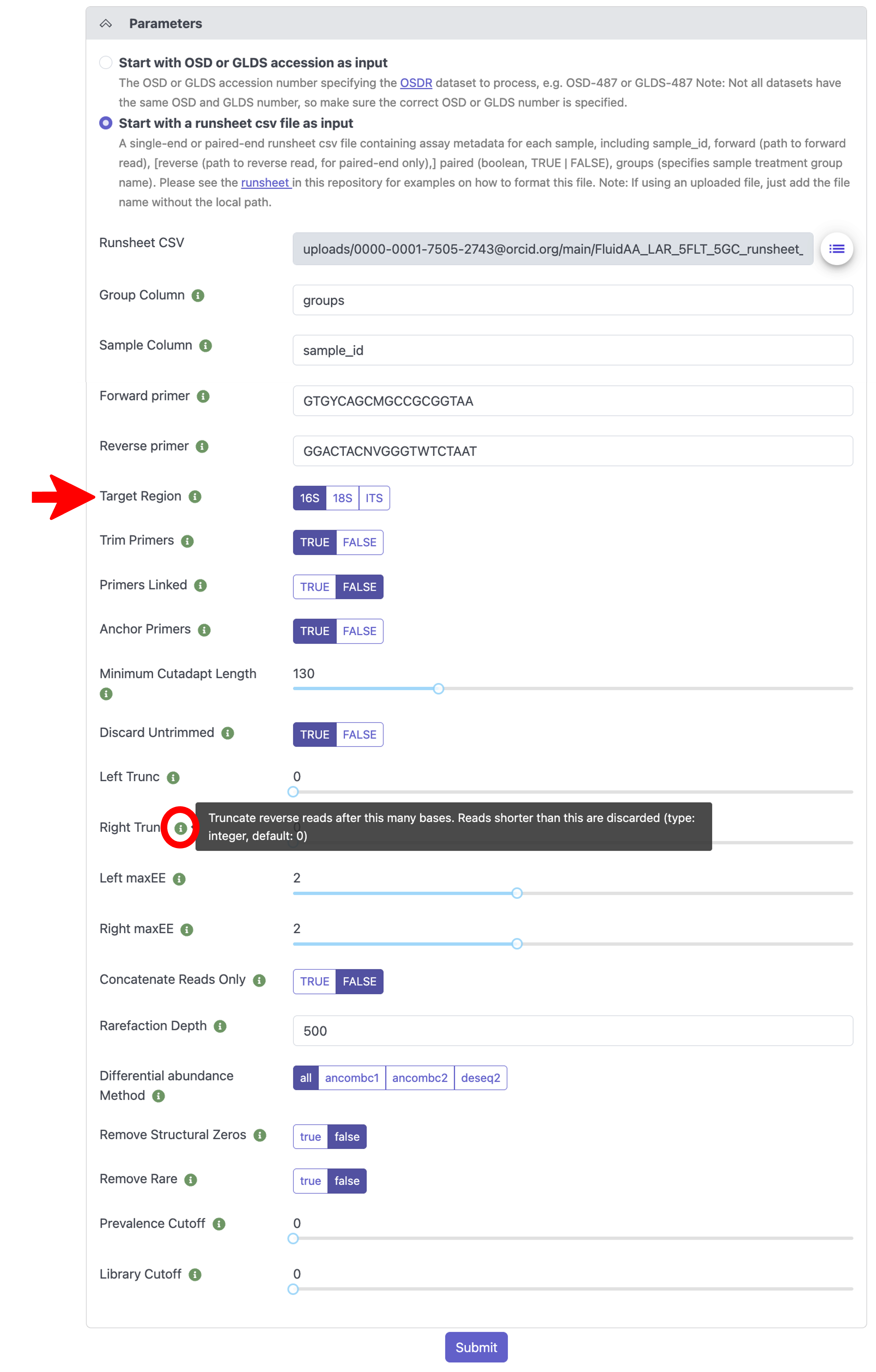
8. Under the “Parameters” section, select the amplicon Target Region that was amplified and sequenced in the dataset you’re processing. All other parameters are set to default values but can be modified. If you are unsure what a specific parameter does, hover over the green “i” icon next to the parameter name for more information, as shown below.

9. When you are satisfied with your parameter selection, click the “Submit” button at the bottom to submit your job to the processing queue.

10. To check the status of your submitted job, following the instructions in the Track, Share, and Modify Projects tutorial.

11. Once your job is complete, you can view and download all output files and visualizations by following the instructions in the View and download output files section below.

View and download output files

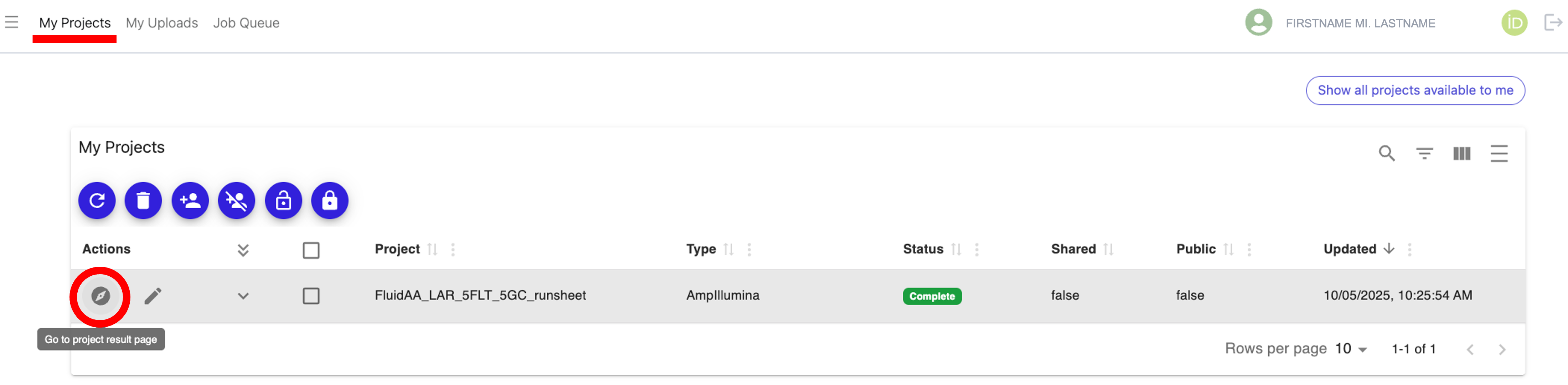
1. Navigate to the “My Projects” tab at the top of the page, find your job (aka project) and check the status to make sure it says “Complete”, then click on the “Go to project result page” icon under the “Actions” column next to your completed project, as shown below:

   Note: If the status of your project is not “Complete”, follow the instructions in the Track, Share, and Modify Projects tutorial to monitor your job status and address any “Failed” projects.

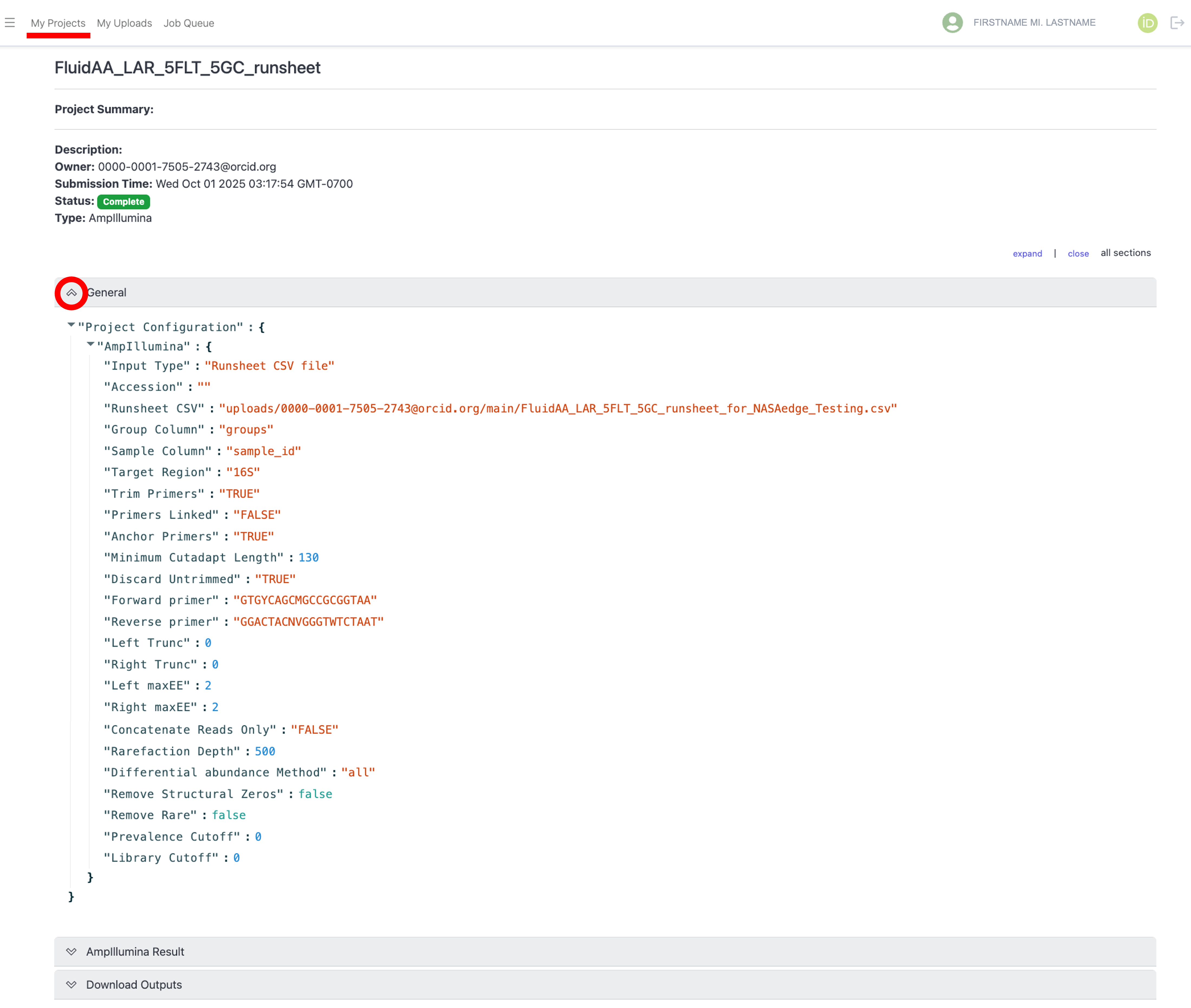
2. On the results page for you project, you will see 3 collapsible bars, “General”, “AmpIllumina Result”, and “Download Outputs”. Click the arrow next to the “General” bar to expand and view the parameters that were used for the project, as shown below:

3. To view the project results, click the arrow next to the “AmpIllumina Result” bar to expand the results, as shown below:

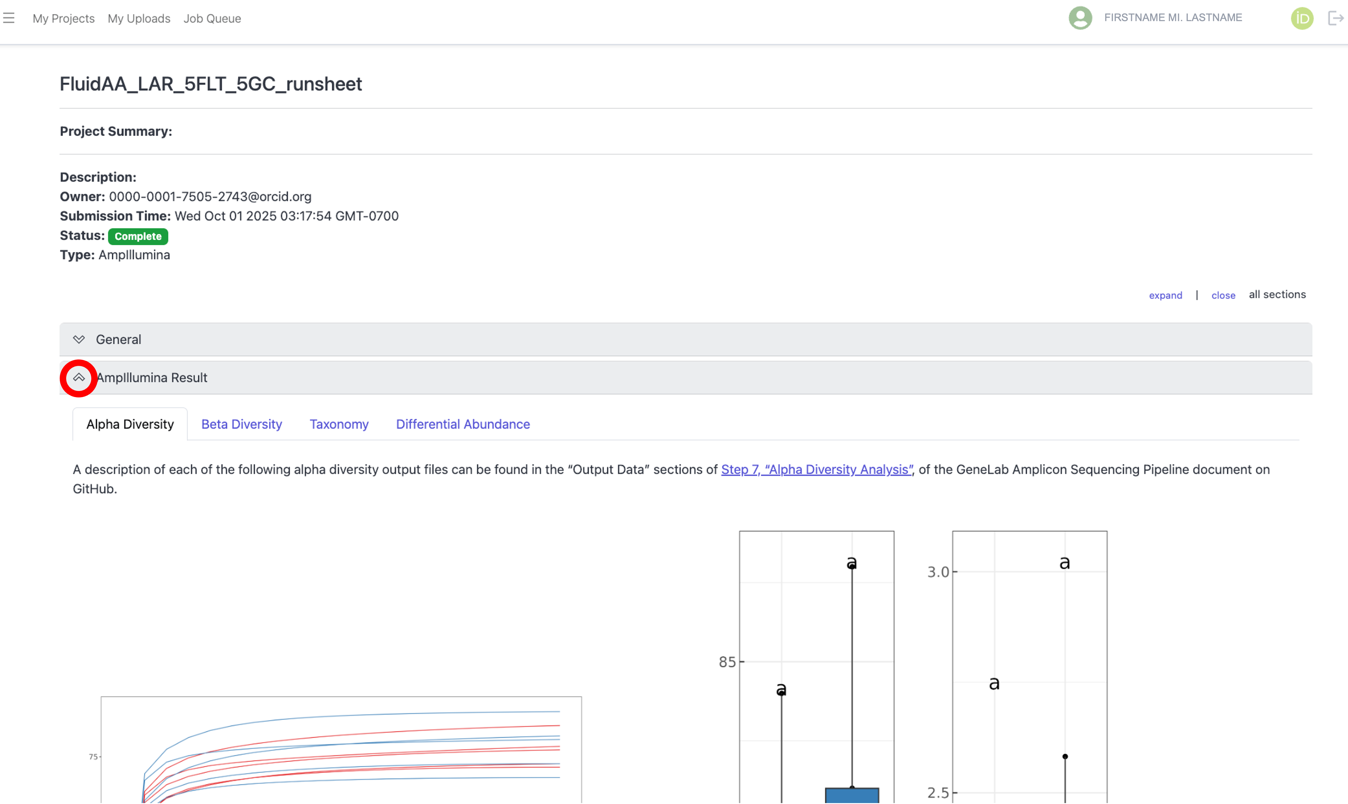
4. To view the alpha diversity results, which examines the variety and abundance of taxa within individual samples, click on the “Alpha Diversity” tab, as shown below:

   Note: A description of each alpha diversity output shown can be found in the “Output Data” sections of Step 7, “Alpha Diversity Analysis”, of the GeneLab Amplicon Sequencing Pipeline document on GitHub.

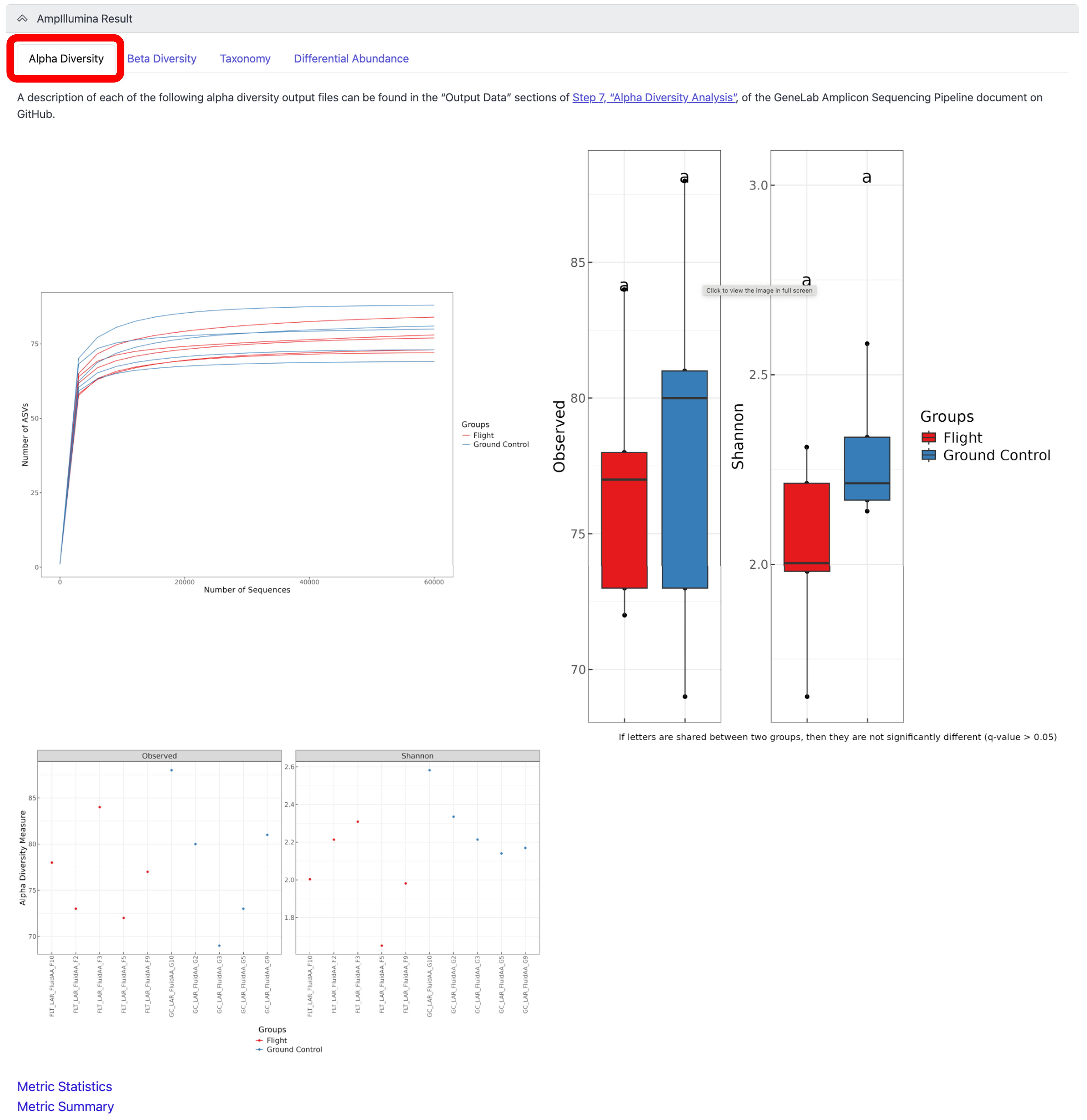
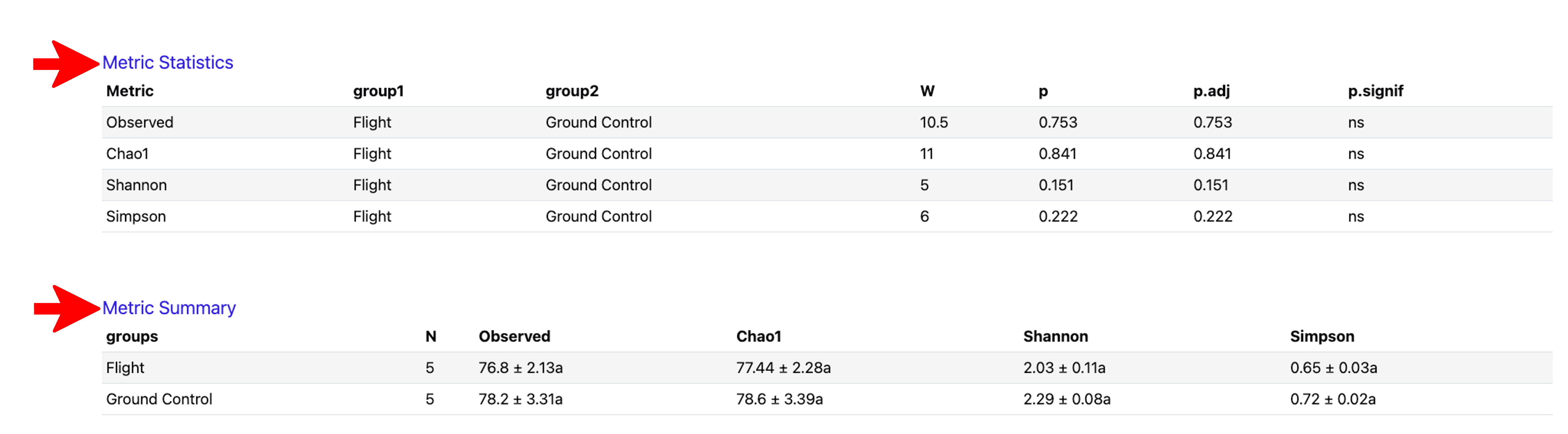
5. Click on the “Metric Statistics” and “Metric Summary” at the bottom of the “Alpha Diversity” tab to view the statistics and summary of the Observed features (i.e. unique taxa) estimates, Chao1 total richness estimates, and the richness and evenness measurements using the Shannon and Simpson indices, as shown below:

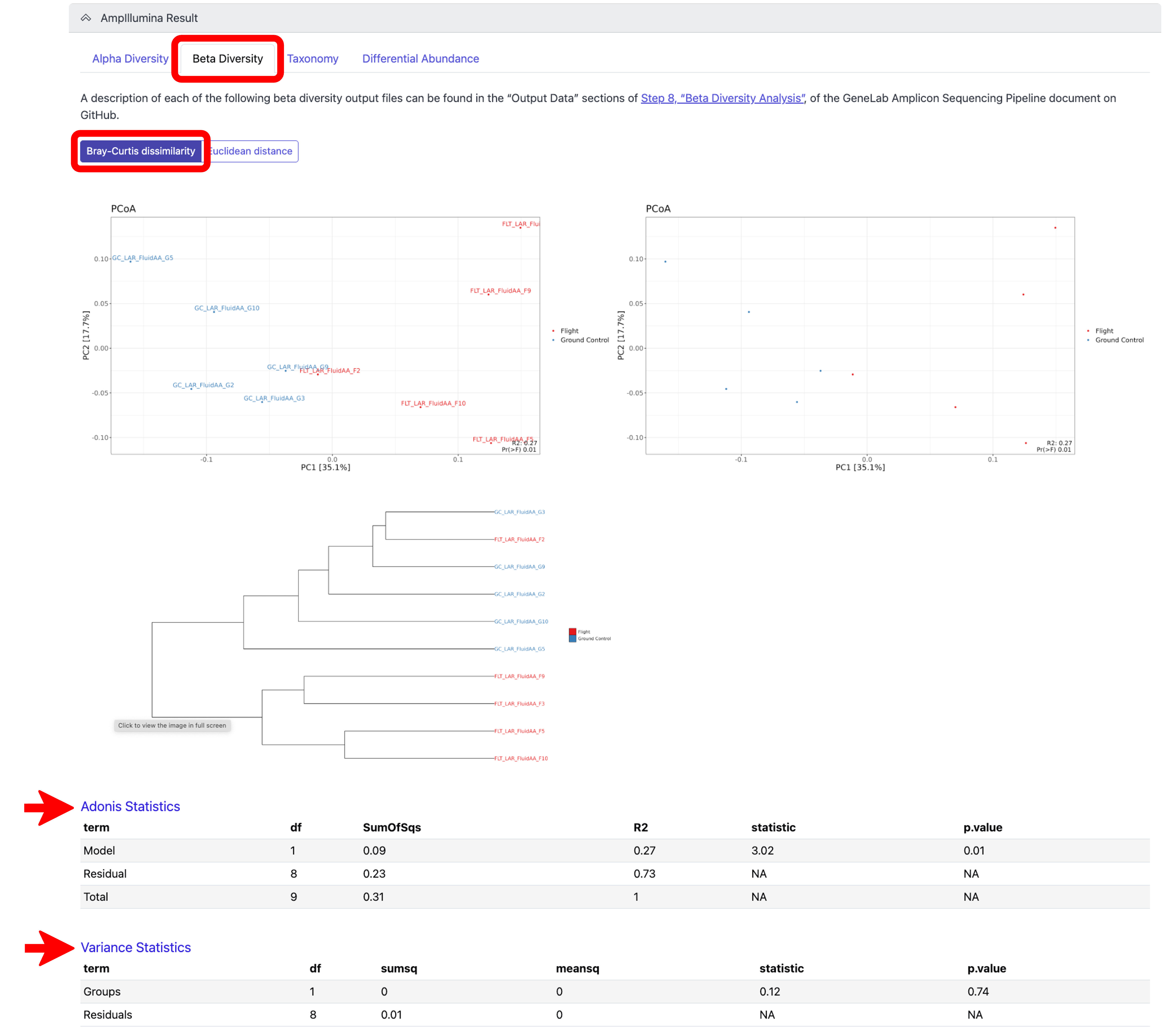
6. To view the beta diversity results, which measures the variation in species composition between different samples or environments, click on the “Beta Diversity Analysis” tab. To view the results after rarefaction normalization, click on the “Bray-Curtis dissimilarity” tab, which used Bray-Curtis dissimilarity to generate dissimilarity matrices for hierarchical clustering, as shown below:

   Note: A description of each beta diversity output shown can be found in the “Output Data” sections of Step 8, “Beta Diversity Analysis”, of the GeneLab Amplicon Sequencing Pipeline document on GitHub. To view the Adonis Statistics and Variance Statistics, click on the respective links at the bottom of the Beta Diversity, Bray-Curtis tab, as shown below.*

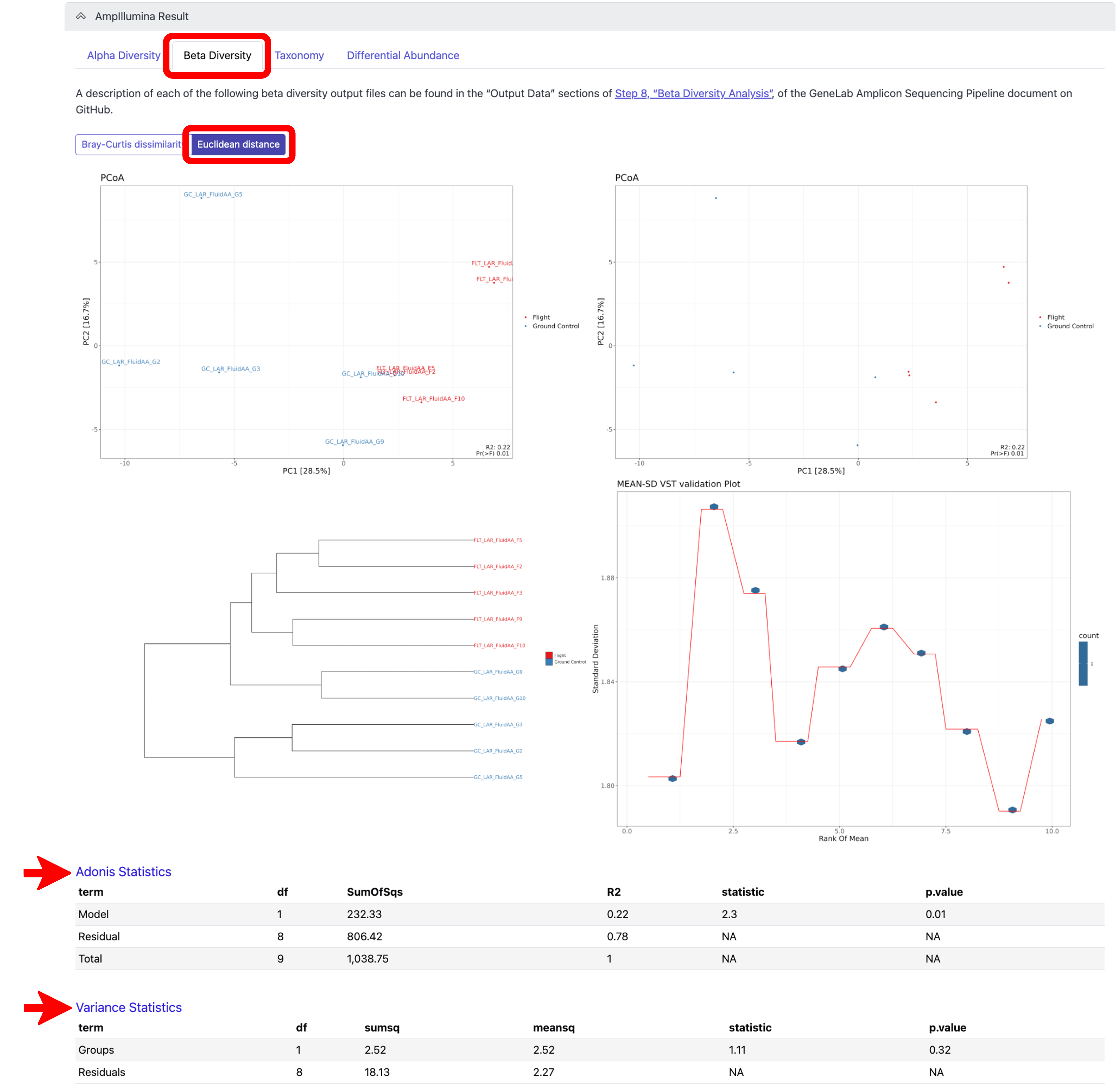
7. To view the beta diversity results after variance stabilizing transformation (VST), click on the “Euclidean distance” tab under the “Beta Diversity Analysis” tab, which used Euclidean distance for hierarchical clustering, as shown below:

   Note: A description of each beta diversity output shown can be found in the “Output Data” sections of Step 8, “Beta Diversity Analysis”, of the GeneLab Amplicon Sequencing Pipeline document on GitHub. To view the Adonis Statistics and Variance Statistics, click on the respective links at the bottom of the Beta Diversity, Euclidean distance tab, as shown below.*

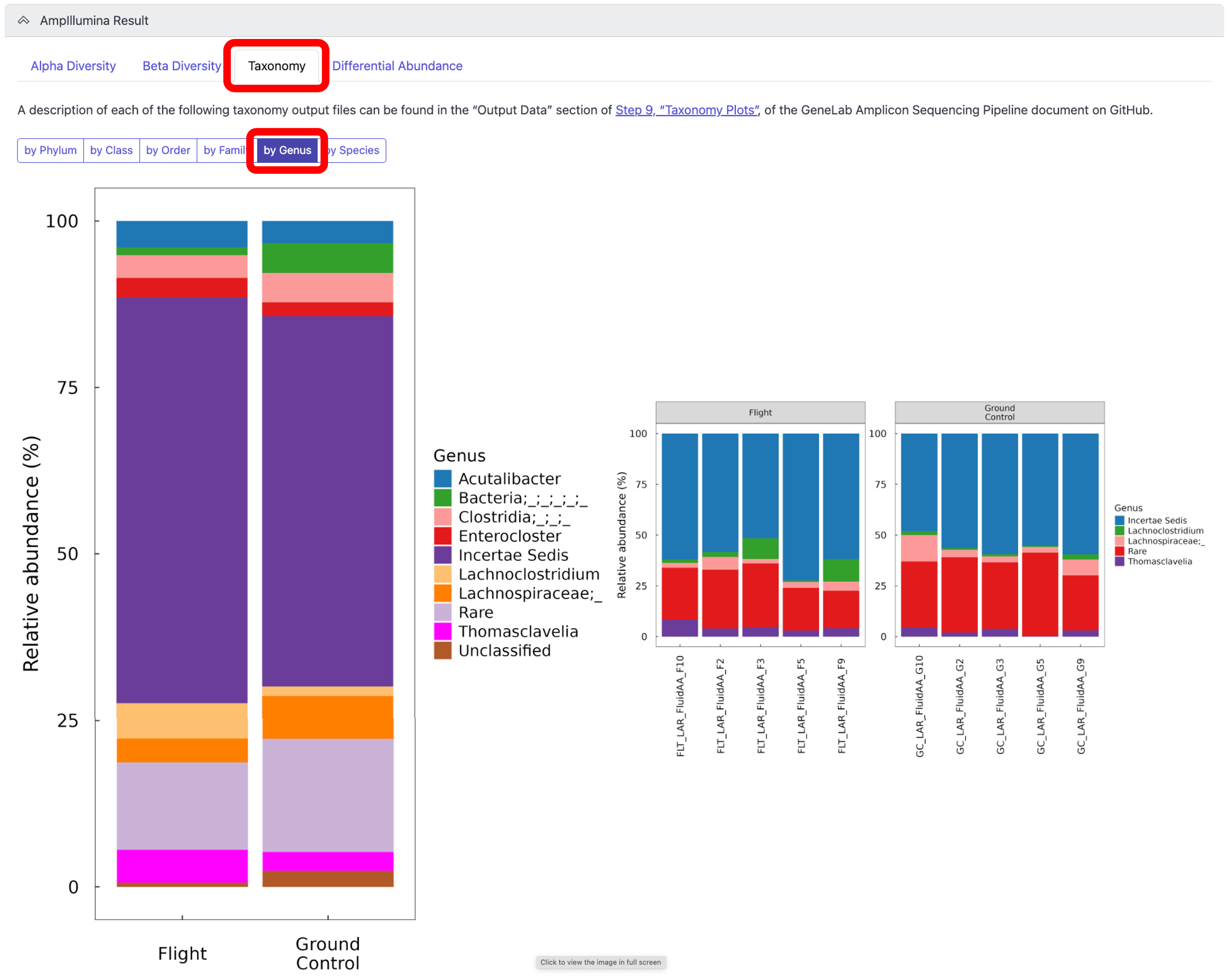
8. To view the relative abundance of taxa at the Phylum, Class, Order, Family, Genus, or Species levels, for both groups and individual samples, click on the “Taxonomy” tab, as shown below:

   Note: A description of each of the taxonomy outputs can be found in the “Output Data” section of Step 9, “Taxonomy Plots”, of the GeneLab Amplicon Sequencing Pipeline document on GitHub. The example below is showing the Genus level relative abundance plots.*

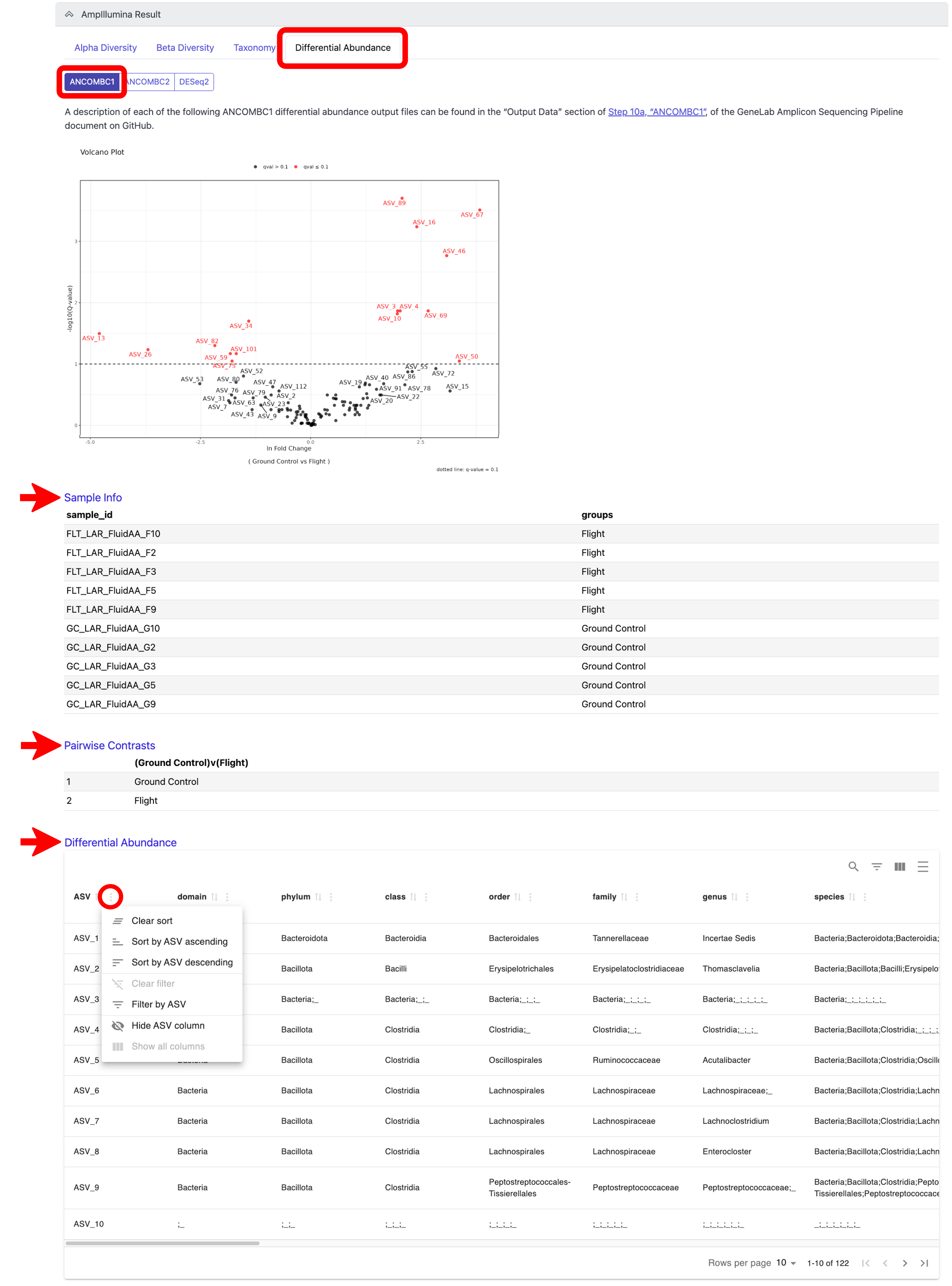
9. Differential abundance analysis is performed using 3 different tools, ANCOMBC1, ANCOMBC2, and DESeq2. To view these results, click on the “Differential Abundance” tab and then on the tab of the tool whose results you want to see. You will be able to view a volcano plot of the differential abundance results for the tool you select for each pairwise group comparison. You can also view the group each sample belongs to by clicking on the “Sample Info” link below the volcano plot(s), and the pairwise comparisons that were evaluated by clicking on the “Pairwise Contrasts” link below the “Sample Info” link; note that both the Sample Info and the Pairwise Contrasts will be the same for all 3 tools. Lastly, you can view an interactive differential abundance table by clicking on the “Differential Abundance” link below the “Pairwise Contrasts” link. The table can be sorted by each column using the sort features displayed when you click the 3 dots next to the respective column, as indicated below; scroll to the right to view all columns. Definitions of each column in the differential abundance tables can be found in the GeneLab GitHub repo, as indicated in the note below. An example of these outputs for ANCOMBC1 is shown below:

   Note: A description of each differential abundance output can be found in the “Output Data” section of Step 10a, “ANCOMBC1”, for ANCOMBC1, Step 10b, “ANCOMBC2”, for ANCOMBC2, and Step 10c, “DESeq2”, for DESeq2 of the GeneLab Amplicon Sequencing Pipeline document on GitHub. Also note that the DESeq2 outputs contain a diagnostic plot of ASV sparsity to be used to assess if running DESeq2 is appropriate.

10. In the expanded “AmpIllumin Result” section, below the part containing the “Alpha Diversity”, “Beta Diversity”, “Taxonomy”, and “Differential Abundance” tabs, you will see the “Read Count Tracking” table, which contains the number of reads for each sample after each step of the pipeline, represented as column headers, with the last column containing the percent of total reads retained after all filtering steps are complete, as shown below. Scroll to the right to view all columns. You can use this table to assess the parameters used for processing. If you notice that a lot of reads are dropped during filtering, you may want to re-process your datasets with less stringent parameters.

    *Note: The table is interactive and can be sorted by each column using the sort features displayed when you click the 3 dots next to the respective column, as indicated below.

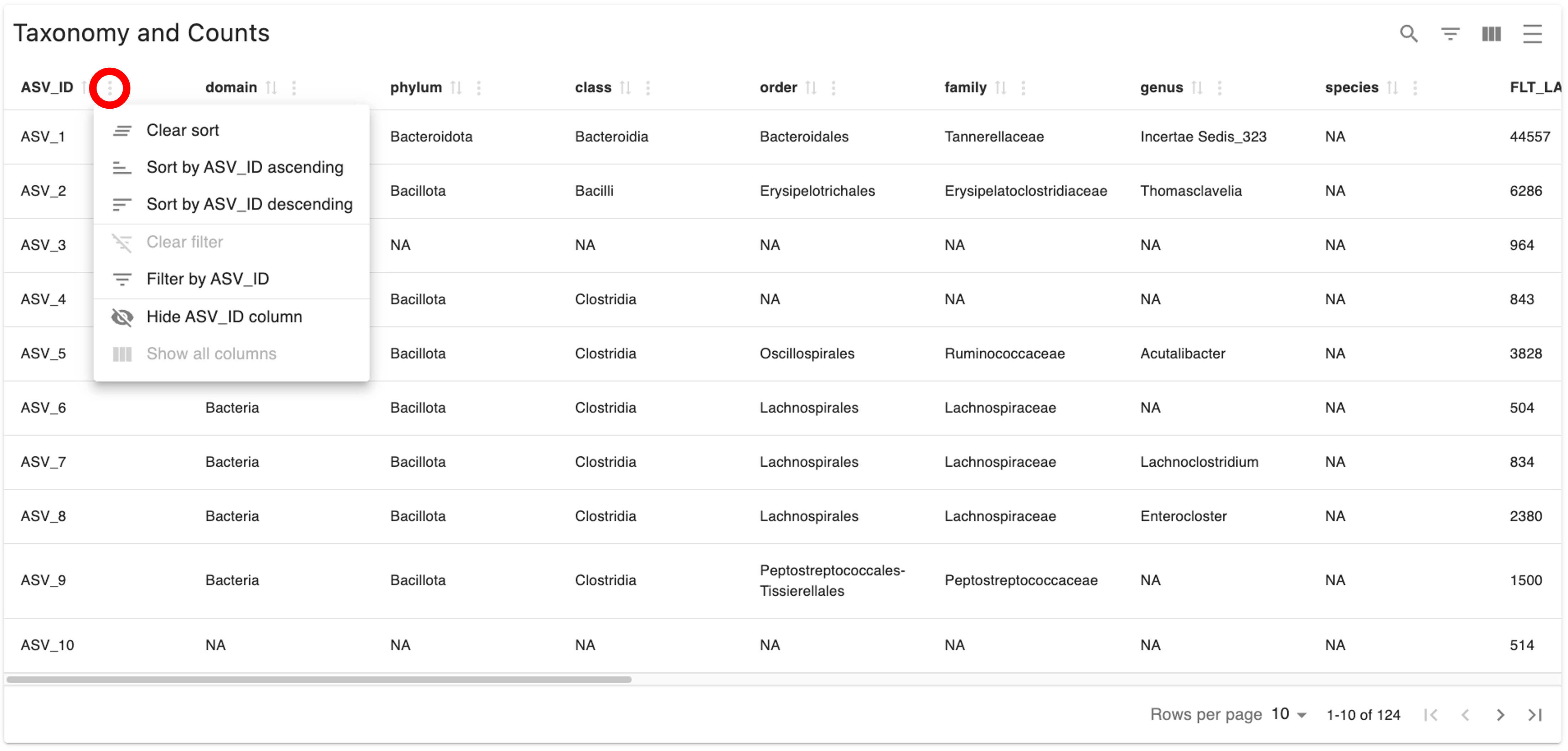
11. In the expanded “AmpIllumin Result” section, below the “Read Count Tracking” table, you will see the “Taxonomy and Counts” table, which contains each amplicon sequence variant (ASV) detected, the taxonomy assigned for each ASV, and the counts of each ASV in each sample in your dataset, as shown below. Scroll to the right to view all columns.

    *Note: The table is interactive and can be sorted by each column using the sort features displayed when you click the 3 dots next to the respective column, as indicated below.

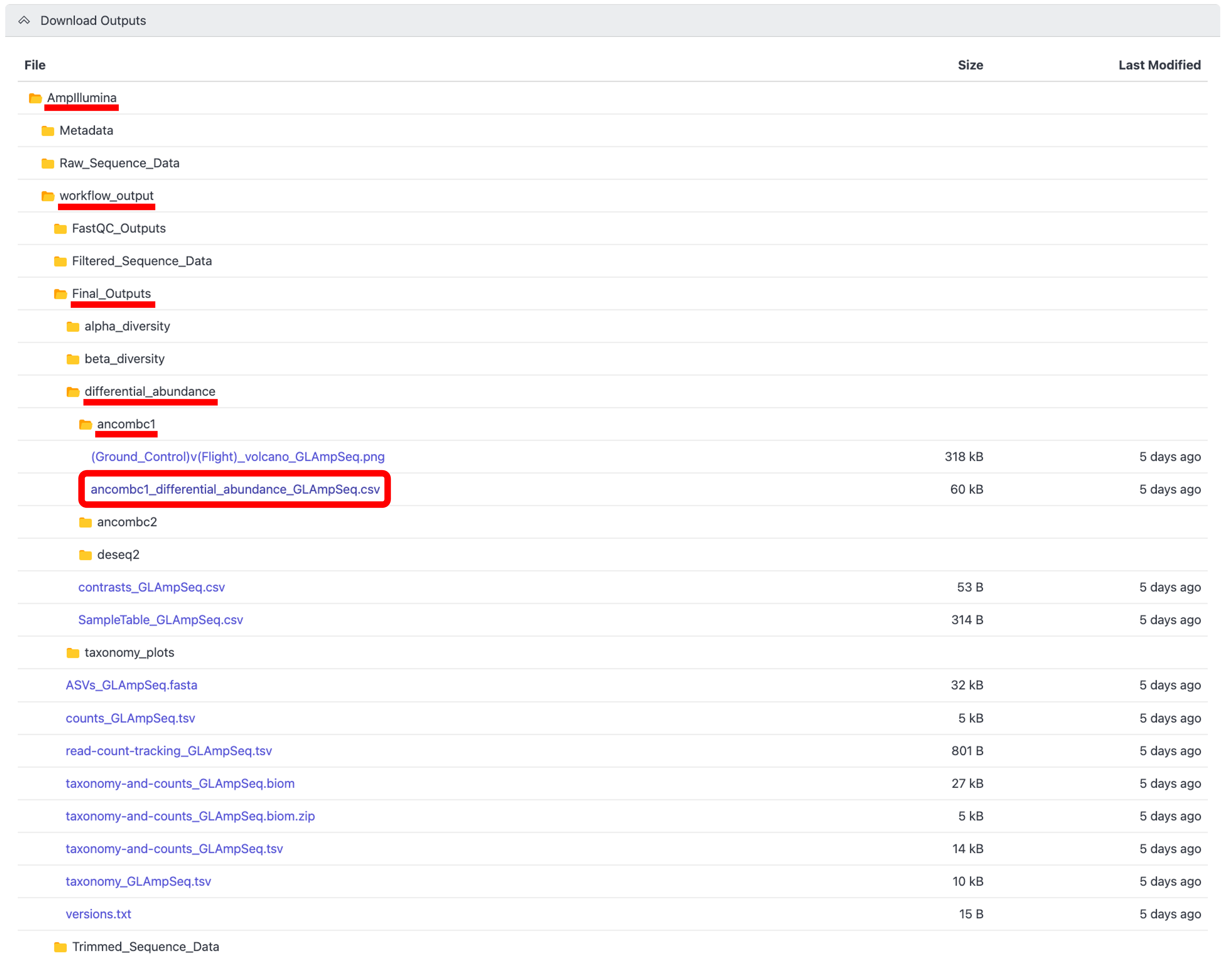
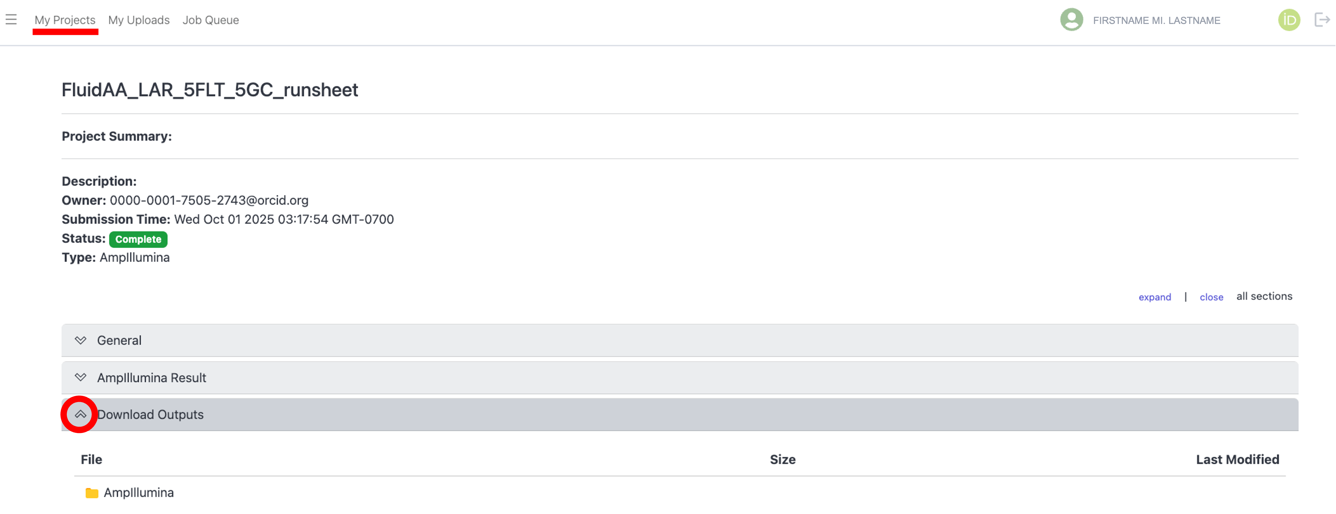
12. To download the output files for the select project, click the arrow next to the “Download Outputs” bar to display the “AmpIllumina” folder containing the downloadable files, as shown below:

13. Click through the folder hierarchy to navigate to the file(s) you want to download, then click on the desired file to download it to your local machine. Below is an example of how to download the ANCOMBC1 differential abundance table.

    Note: Only individual files can be downloaded.